Macro Placement with Reinforcement Learning

Summary

In 2021, Google researchers reported that a reinforcement-learning agent could produce chip floorplans as good as or better than human experts' in under six hours (Mirhoseini, Goldie, et al., Nature 2021, with open-source code in Circuit Training). This project rebuilds that method from scratch at laptop scale, in six versions. Each version adds one piece of the paper and is measured against random placement on the same problems. The goal was to understand each piece of the method by building it, and to find out which pieces actually help at this scale.

In short: the learning works, but learning to place well on new problems is hard. On one fixed problem, the agent learns a layout that beats 90 percent of random ones. On 200 problems it has never seen, it is only 2.6 percent better than random, and adding the paper's graph network and spatial output layer did not change that. See the results.

The problem

A chip is built from two kinds of blocks. Macros are large fixed blocks, such as memories, that each take up a big rectangle of the chip. Standard cells are the small logic gates that make up the rest, often millions of them. Wires called nets connect them. Where the macros go decides how long those wires must be and how crowded the chip becomes. This step, macro placement, is still largely done by hand, and the paper notes that it takes human experts several weeks for each block of a modern chip.

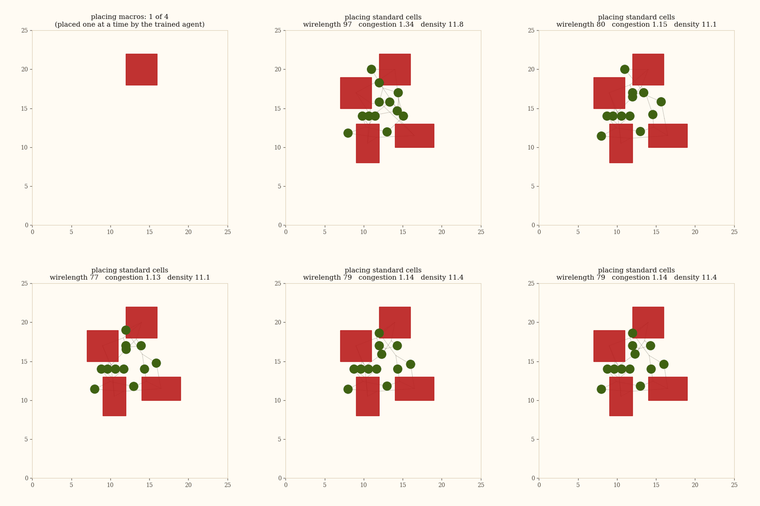
The paper turns it into a game played on a grid laid over the chip. An agent places the macros one at a time, each on a grid cell, and may not pick a cell where the macro would overlap another or hang off the edge. Once every macro is down, a fixed rule places the standard cells, which are grouped into clusters to keep their number manageable. The finished layout then gets one score, and that score is all the agent learns from.

The problems here are small. Most versions place 4 macros and 12 clusters on a 25 × 25 grid, and the scaling study goes up to 14 macros. The paper's designs have tens to hundreds of macros and millions of standard cells. They are kept small so that each version trains in an hour or less on one laptop, because every episode runs the cell placement and scoring on the processor.

How the standard cells are placed

The clusters are placed by force-directed placement, which works like objects joined by springs, sliding until the forces balance. Three forces act on each cluster.

The clusters take 60 small steps under these forces, and a final clean-up pass makes sure no cluster is left on a macro. These are V2's settings. V3 onward use an earlier version of the rule, noted under V3 below.

How a layout is scored

The true test of a layout is a full place-and-route run, which takes minutes to hours. Training needs tens of thousands of layouts, so the paper scores each one with three fast estimates, which it calls proxies. In V2, a whole episode, including the cell placement and the scoring, takes about 16 milliseconds.

Lower is better for all three.

The three scores are combined into one cost, and the reward is its negative.

cost = 0.1 \cdot W + 10 \cdot C + 2 \cdot D

reward = - cost

$W$: total wirelength (about 80 to 150 on these problems)
$C$: congestion (about 1.1)
$D$: density (about 11)
$0.1, 10, 2$: weights that set how much each score counts. With these values, density makes up about half of the total cost

How the agent learns

Think of learning a video game with no instructions. You press buttons, see what happens, and watch your score. Over many games you repeat what tended to raise the score and drop what did not. Reinforcement learning is that process, run by a computer for thousands of rounds.

Agent

The decision-maker.

Here: a neural network.

State

What the agent can see when it decides.

Here (in V1): which cells are taken, where the next macro's connected neighbors sit, and which macro is next.

Action

One choice the agent makes.

Here: the cell where the next macro goes.

Reward

A number saying how good the outcome was.

Here: minus the layout's cost, so cheaper layouts score higher.

Episode

One complete attempt, start to finish.

Here: placing every macro once.

Policy

The agent's strategy: how likely it is to pick each action in each state.

Training changes this.

Why each piece is there

All four of these choices are taken directly from the paper, and every version keeps them.

01

Mask illegal moves, do not penalize them

What: illegal cells are removed before the agent chooses, using MaskablePPO (Maskable Proximal Policy Optimization) from sb3-contrib.

Why: a penalty only discourages overlap. A mask makes it impossible, so no training time is spent learning the rule.

02

One macro per step

What: place one, look, place the next.

Why: a few small decisions are far easier to learn than one giant one.

03

One reward, at the end

What: no score until the layout is complete.

Why: a floorplan is only good or bad as a whole. The cost: the agent must work out which moves earned the score.

04

A grid of choices

What: the action is a grid cell (625 options on a 25 × 25 grid).

Why: a fixed list of choices makes masking easy. The cost: positions snap to the grid.

How the agent gets better

The policy starts out random. Over thousands of episodes, training shifts probability toward the choices that led to cheaper layouts. The method that decides how to make each shift is Proximal Policy Optimization (PPO), the same one the paper uses.

How training works, step by step: from policy gradient to Proximal Policy Optimization (PPO)

Each bar is the chance of placing the next macro in one candidate cell.

The policy starts out random. Inside, it is a small neural network controlled by tens of thousands of adjustable numbers (81,936 in V1), written θ (theta). Think of them as knobs: turn them and the probabilities change. A training method is a rule for which way to turn the knobs after each batch of episodes, and how far. There are two broad families of rules.

Each step on the right keeps everything above it and fixes one weakness.

The math, step by step

The other family

Value-based: Q-learning (Q for quality)

Keep a score for every action in every state: how much reward to expect after taking it. Play by taking the highest-scoring action. After each move, nudge that score toward what actually happened.

Q (s, a) \leftarrow Q (s, a) + α [r + γ max_{a^{'}} Q (s^{'}, a^{'}) - Q (s, a)]

$Q (s, a)$: the score: expected future reward for action a in state s
$α$: step size: how big each nudge is
$r$: the reward just received
$γ$: how much future reward counts compared with reward now
$max_{a^{'}} Q (s^{'}, a^{'})$: the best score available from the next state

The strategy is only implied: always take the top score. The paper learns the strategy itself, so this project does too.

Step 1

Policy gradient: learn the probabilities directly

Skip the scores. After an episode, turn the knobs so each choice becomes more likely in proportion to the score that followed it.

θ \leftarrow θ + α \cdot G \cdot \nabla_{θ} \log π_{θ} (a | s)

$θ$: the knobs: every adjustable number in the network
$π_{θ} (a | s)$: the probability the policy gives action a in state s
$\nabla_{θ} \log π_{θ} (a | s)$: which way to turn each knob to make action a more likely (the log points the same way and keeps the math simple)
$G$: the score that followed this choice. Here: minus the final cost
$α$: step size: how far to turn

Still a problem: here every score is negative, because it is minus the cost. So every choice gets pushed down, only by different amounts. Learning is slow and noisy.

Step 2

Actor-critic: judge each choice against what was expected

Add a second small network, the critic, that looks at the state and predicts the score the episode will end with. The policy is now called the actor. Each choice is judged by how much better or worse things went than the critic predicted.

A = G - V (s)

θ \leftarrow θ + α \cdot A \cdot \nabla_{θ} \log π_{θ} (a | s)

$V (s)$: the critic's prediction: the score it expects from state s. The critic is trained alongside the actor to predict better
$A$: the advantage: positive if the episode beat the prediction, negative if it fell short

Fixes: better-than-expected choices go up and worse ones go down, even when every score is negative. Still a problem: nothing limits how far one update turns the knobs. One lucky batch can make a mediocre move look great, and a big overreaction can wreck what thousands of episodes taught.

Step 3: used here

Proximal Policy Optimization (PPO): limit each update

"Proximal" means "nearby": each update must keep the new policy close to the old one. Measure how much each choice's probability has changed with a ratio, and stop rewarding change beyond a small band.

ρ = \frac{π_{θ} (a | s)}{π_{old} (a | s)}

L = \min (ρ A, clip (ρ, 1 - ε, 1 + ε) A)

$π_{old} (a | s)$: the probability before this update began
$ρ$: the ratio: 1.0 means unchanged, 1.2 means 20 percent more likely
$ε$: the allowed band. Here 0.2, so the ratio is capped between 0.8 and 1.2
$clip$: holds the ratio inside that band
$\min$: takes the more cautious of the two versions
$L$: the objective. Training turns θ to make it as large as possible

Fixes: no single update can move far, so one noisy batch cannot undo past learning. Because each step is safe, every batch is reused for 10 passes instead of being thrown away after one.

Training turns θ to make L larger. Where the line is flat, turning θ cannot raise L any further, so that choice stops being pushed for the rest of this batch.

An earlier method, Trust Region Policy Optimization (TRPO), enforced a similar limit with much heavier math. Proximal Policy Optimization (PPO) gets most of the benefit with a simple clip, which is why it became the standard. In this project each batch is 2,048 placements, and the code uses a smoothed form of the advantage called Generalized Advantage Estimation (GAE); the idea is the same.

The six versions

Each version keeps everything before it and adds one piece of the paper, so that each piece's effect can be measured on its own. The results for all six follow in the next section, and the learning method itself is explained after that.

V1: the learning loop

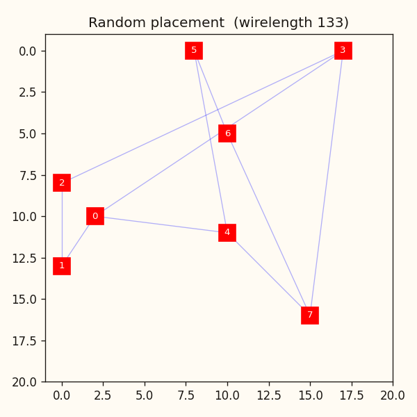
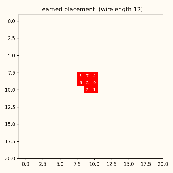
The loop in its simplest form: eight macros, each a single cell, on a 20 × 20 grid, with no standard cells. The reward is minus the total wirelength. V1 trains and is tested on one fixed problem, so it can memorize the answer. That is deliberate: it proves the machinery before asking it to generalize.

The agent sees the two grids, plus which macro is next. Input 2 is the strong hint: it shows where the next macro's connections already sit. In V1 every macro fills a single cell, so the mask only removes cells that are already taken. From V2 on, macros have real sizes and the mask checks the whole footprint.

Each step places one macro (outlined: the newest) and earns nothing. Only the finished layout is scored, and that one score judges all eight choices.

V1 source on GitHub →

V2: the paper's score

Three changes bring the problem in line with the paper. The macros get real sizes: four rectangles (4 × 4, 3 × 5, or 5 × 3 cells) on a 25 × 25 grid, and the mask now allows a corner only if the whole rectangle fits without overlapping another macro. Twelve clusters of standard cells are added and placed by the force-directed rule. The reward becomes the three-part cost. The agent and its training settings are unchanged, and it still trains and is tested on one fixed problem.

One V2 episode. The line under each stage is what V2 adds to V1. Times are averages over 200 episodes of the trained V2 agent on one processor thread, not counting the learning updates. Stages 2 and 3 grow with the number of clusters and nets, which is why the problems are kept small.

V2 source on GitHub →

V3: a new problem every episode

From solving one problem to learning a placer. Each episode now starts with a fresh random problem: every macro gets a random width and height between 3 and 5 cells, every cluster a random area, and the connections are redrawn. The number of macros and clusters stays fixed, so the agent's inputs and choices keep the same shape, and two extra inputs tell it the current macro's width and height. Training and test problems come from two separate random streams, so no test problem is ever seen in training.

Real problems from the generator, with each problem's four macros drawn to scale. Only the sizes and the connections change: there are always four macros and twelve clusters.

A note on cell placement V3 and the later versions use an earlier version of the cell-placement step than V2. Its clusters start at the center of the grid rather than among the macros, every pair of clusters pushes apart however far apart they are, and the final clean-up runs once and keeps clusters about half a cell clear of a macro instead of a full cell.

V3 source on GitHub →

V4: the netlist as a graph

V4 lets the agent see the whole netlist. Up to V3, its only clue about wiring is which placed macros share a net with the next one. But nearly every net includes a cluster, so most links between macros pass through a cluster, and V3 never sees them.

The same three objects as each version sees them. V3 only knows which placed macros share a net with the next macro, so links that pass through a cluster are invisible to it.

To show it everything, V4 draws the netlist as a graph, the central idea of the paper. Every macro and cluster is a point, a line joins two objects that share a net, and each object carries eight numbers about itself.

Squares are macros and dots are clusters. A line joins two objects that share a net. Some clusters are left out for clarity.

A graph network then condenses the graph into a few numbers the agent can use. It works in rounds, like news passing between friends: in each round, every object blends its numbers with its neighbors' numbers. After two rounds, the macro about to be placed has heard from objects up to two connections away, which is enough to see that A, c and B belong together.

One action. Macros 1 and 2 are already on the chip, and the agent must now place macro 3 (outlined). Clusters are placed only after every macro, so for now they exist only in the graph. Each line is a shared net.

A real action from the trained V4 agent on one of the 200 test problems. The macro sizes and positions, the nets and the glow strengths (the network's averaging weights, before the learned layer

W

) are the actual ones. Only the positions of the unplaced objects on the right are chosen for drawing.

The math: one round of mixing

H^{new} = ReLU (\hat{A} H W)

$H$: every object's numbers, one row per object
$\hat{A}$: who connects to whom, including each object to itself, scaled so that heavily connected objects do not drown out the rest
$W$: learned weights, separate for each round. They describe no particular graph: the same $W$ is applied to every object, in every problem. It is a recipe that turns each object's mixed numbers into new ones, each new number a weighted blend of the old ones (8 numbers become 32 in round 1, and 32 stay 32 in round 2). Training tunes the recipe so that the new numbers carry whatever helps the agent place macros well.
$ReLU$: Rectified Linear Unit (ReLU): keeps positive values and sets negative ones to zero

The rest of the agent is unchanged from V3. The graph's summaries are simply added to what it already sees.

The graph network only adds the top path. The grid path and the layers that score the 625 cells work as in V3.

The graph network is small, only 1,344 adjustable numbers. Most of the policy's 110,961 still sit in the grid summary and in the layers that score the 625 cells.

V4 source on GitHub →

V5: a spatial output layer

V5 changes only the agent's very last step: turning its summary of the situation (64 numbers) into 625 scores, one per cell of the grid. The macro goes to the best-scoring cell it fits in.

V4 does this with a plain layer, which gives every cell its own private set of weights. Picture a theater with a separate judge for each of its 625 seats, each judge with their own rulebook. Seats 12 and 13 are almost the same seat, yet what judge 12 learns teaches judge 13 nothing, so every judge has to learn on their own.

A convolution replaces the 625 rulebooks with one small rule card. The card looks at a 3 × 3 patch, a cell and its eight neighbors, and is slid across the whole grid, so every cell is scored the same way. A lesson learned at one spot now applies everywhere, and neighboring cells, whose patches overlap, get similar scores.

A small corner of the 25 × 25 grid. On the left, each shade stands for one cell's private weights. On the right, the card scores the dark center cell from the 3 × 3 patch around it, then moves on. Neighboring cells share most of their patch, so they get similar scores.

The paper builds its grid of scores with deconvolution layers. A deconvolution works the other way round from a convolution: it grows a small picture into a bigger one, like enlarging a thumbnail, with learned weights filling in the detail. The paper starts from a tiny map and doubles it five times. V5 takes a simpler route to the same end, called a spatial head here: it turns the 64 numbers into a small 5 × 5 map, stretches that to 25 × 25 by plain resizing, then runs convolutions over it.

V5 placing macro 3, on the same test problem as the figure above (macros 1 and 2 are outlined on the right). Everything starts from the agent's summary of the situation: 64 numbers.

The real values from the trained V5 agent on one of the 200 test problems. From step 3 on, the maps are shown averaged over their 32 layers, and darker means larger. Each score depends only on the 3 × 3 patch around its cell, across all 32 layers: the 3 × 3 convolution and the final 1 × 1 convolution act together as one card.

V5 source on GitHub →

V6: a scaling study

V3 to V5 all use four macros. The paper's designs are far larger, so V6 asks whether the graph policy pulls ahead as problems grow. The number of macros, the number of clusters and the grid all grow together, and macro sides grow with the grid, up to a sixth of its width.

Macros	Clusters	Grid	Cells to choose from
4	12	25 × 25	625
6	18	31 × 31	961
8	24	35 × 35	1,225
10	30	40 × 40	1,600
12	36	43 × 43	1,849
14	42	47 × 47	2,209

Two policies are trained at every size. The graph policy is V5's design. The flat policy gets exactly the same inputs but reads them as one long list with ordinary layers, with no message passing and no spatial head, so it is not V3's flat-grid policy. Every run gets the same budget of 100,000 placements, a third of V3's, so larger problems get fewer episodes: 25,000 at 4 macros, but only 7,142 at 14. The test is also lighter: each size is tested on 40 unseen problems, and each problem is compared with a single random layout, not 100.

V6 source on GitHub →

Results

Version	Tested on	Learned cost	Random average	Better than random by	Random layouts it beats
V1	One fixed problem	12 (wirelength)	133 (wirelength)	91 percent	All 2,000
V2	One fixed problem	42.1	44.7	5.8 percent	90 percent
V3	200 unseen problems	44.1	45.2	2.6 percent	70 percent
V4	The same 200	44.1	45.2	2.4 percent	70 percent
V5	The same 200	44.3	45.2	2.1 percent	67 percent
V6	40 unseen problems at each of 6 sizes	Flat and graph policies, 4 to 14 macros		−0.9 to +2.7 percent	Within the noise

Lower cost is better. Cost is the weighted sum of wirelength, congestion and density; V1 is scored on wirelength alone. Random placement drops each macro on any allowed cell, on the same problems. "Random layouts it beats" compares the learned layout with every random layout drawn for the same problem.

One fixed problem: the loop works (V1 and V2)

V1, scored on wirelength alone, packs connected macros tightly together. Its layout needs about a tenth of the wire of an average random one.

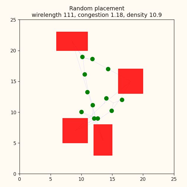
A random placement: macros scattered across the grid with long crossing nets. — Random (a typical example, close to the average of 2,000 random layouts): wirelength 133.

The learned placement: macros gathered into one tight overlap-free cluster. — Learned: wirelength about 12, with zero overlaps.

V2, scored the paper's way, has a lower total cost than 90 percent of 1,000 random layouts. It gets there by trading: much shorter wires, the same congestion, and slightly worse density.

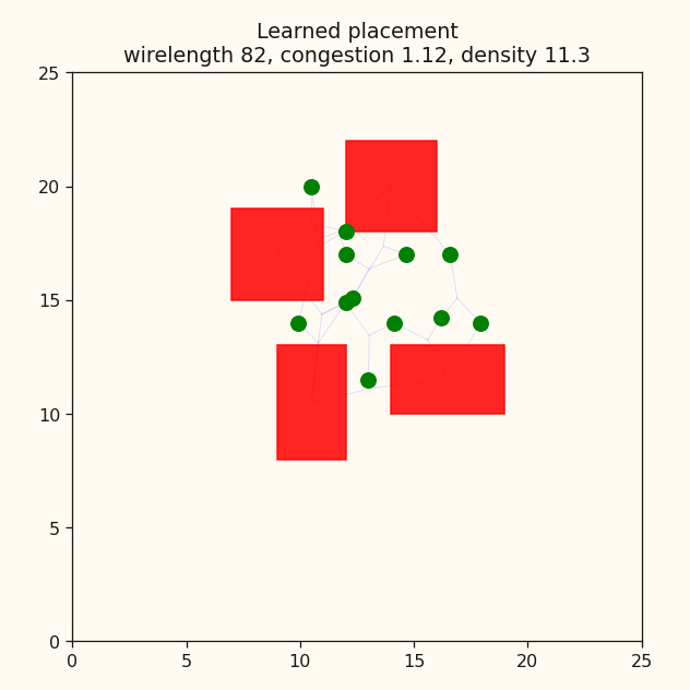
A random macro placement with clusters and nets around it. — Random (a typical example, with a total cost close to the random average): wirelength 111, congestion 1.18, density 10.9.

The learned macro placement with macros grouped around the clusters. — Learned: wirelength 82, congestion 1.12, density 11.3. Red: macros. Green: cell clusters. Faint lines: nets.

Score (lower is better)	Random average	Learned	Learned beats
Wirelength	117	82	98 percent of random
Congestion	1.11	1.12	47 percent of random
Density	10.9	11.3	19 percent of random
Total cost	44.7	42.1	90 percent of random

The trade follows from the problem. The four macros hold more area than all twelve clusters combined (62 cells against 50). Packing them together saves a lot of wire, but it also crowds the busiest bins, which raises density. Of the three weighted terms, wirelength changes the most from one layout to another, so it is where the agent has the most to gain.

A robustness check confirms that this result is not an artifact of chance. The force-directed step starts from a random seed, and training always used the same one. Rescored with 20 other seeds, the learned layout still beats random 95 percent of the time.

Unseen problems: a small gain, unchanged by the paper's architecture (V3 to V5)

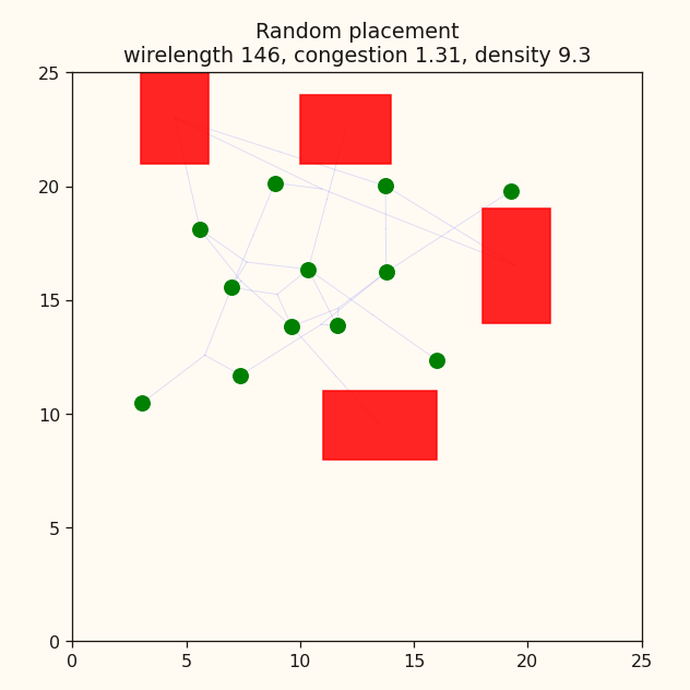
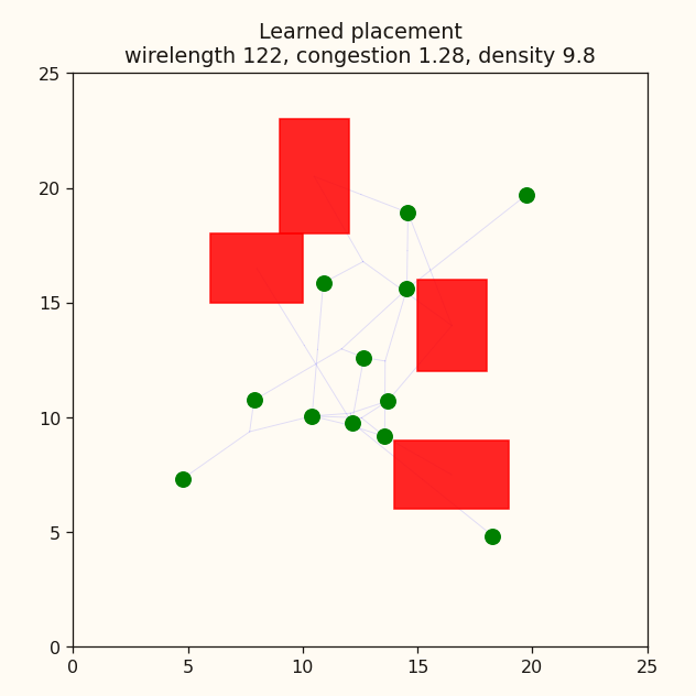
V3, V4 and V5 were each tested on the same 200 unseen problems, against the same 100 random layouts per problem.

A random macro placement on a test problem, with clusters and nets around it. — Random (a typical layout, with a cost close to the random average): wirelength 146, congestion 1.31, density 9.3.

The learned macro placement on the same test problem, with the macros grouped closer around the clusters. — Learned: wirelength 122, congestion 1.28, density 9.8. The agent never saw this problem in training, and its gain here is the median gain across the test problems.

Score (lower is better)	Random average	V3 (flat)	V4 (graph)	V5 (graph, spatial head)
Wirelength	123	114	114	115
Congestion	1.14	1.13	1.14	1.13
Density	10.8	10.7	10.7	10.7
Total cost	45.2	44.1	44.1	44.3
Share of random layouts beaten		70 percent	70 percent	67 percent

V3's gain over random is real but small, and almost all of it is shorter wiring: its congestion and density are no better than chance. It is not memorizing, because it scores about the same on 200 problems it trained on (44.2) as on unseen ones (44.1). The graph network (V4) and the spatial head (V5) made no measurable difference: V4 beats V3 on 99 of the 200 problems, a coin flip, and V5 beats it on 92, within the margin of error.

Limits Keeping the cheapest of 100 random layouts beats V3 on 191 of the 200 test problems, V4 on 191 and V5 on 197. Each version was trained once, so small differences between versions could be run-to-run variation.

Why: one fixed arrangement

None of the three policies reads the problem much. On the 200 test problems, V4 put its first macro on the same cell every time, and its second macro on the same cell in 153. V5 holds its arrangement even more firmly: 194 and 195. V3 behaves the same way. Deleting all of the netlist's connections from V4's input never changes its first move, and changes 366 of its 800 moves in total. Each has learned one good general arrangement, not a way to adapt to the problem in front of it, so a better view of the problem has nothing to work with.

Does the graph policy pull ahead with size? (V6)

The study ran twice. The first run (3 sizes, 25 test problems, and very slightly different 8- and 14-macro problems) showed the graph policy rising with size, from 1.3 to 2.0 to 2.4 percent better than random, which looked like the paper's advantage appearing. The second run (6 sizes, 40 test problems) did not show it. The flat policy came out ahead at all six sizes, and both policies fell toward random as the problems grew.

Error bars show about ±1.1 points, the spread that comparing with a single random layout per problem causes on its own (measured on 4-macro problems). They leave out variation between training runs, which the two 4-macro results show is at least as large.

The numbers behind the chart

Macros	Flat, second run	Graph, second run	Flat, first run	Graph, first run
4	+2.6	+2.7	+2.1	+1.3
6	+1.6	+1.3
8	+2.4	+0.1	+0.5	+2.0
10	+1.3	+0.3
12	+1.1	+0.1
14	−0.3	−0.9	+1.7	+2.4

Each number is the percentage by which the policy's average cost is lower than random placement's, on that size's test problems. Positive means better than random, negative means worse. Flat and graph are the two policies, and blank cells are sizes the first run did not test.

It is tempting to read the second run as refuting the first, but neither run is precise enough to settle anything. Comparing each problem with a single random layout moves each number by up to about 1.1 points on its own, and the gap between the two policies by about 1.6. Training once per point adds at least as much: at 4 macros, with identical settings and test problems, the graph policy scored 1.3 percent in one run and 2.7 in the other. Against that noise, the first run's rising line is not a real trend, and in the second run only the 8-macro gap (2.3 points) clearly exceeds the margin.

What V6 can and cannot say At this training budget, run-to-run noise is as large as any difference between the policies, so this study cannot tell whether the graph policy pulls ahead with size. It also starves the larger problems: at 14 macros each run sees under a third as many episodes as at 4, while choosing among more than three times as many cells. A fair test needs several training runs per point, many random layouts per problem, and a training budget that grows with problem size.

Compared with the paper

The paper's details are from its arXiv version.

Aspect	The paper	This project
Learning method	Proximal Policy Optimization (PPO), one macro per step, illegal cells masked, one reward at the end	The same, in every version
Design size	Tens to hundreds of macros, millions of standard cells	4 to 14 macros
Standard cells	Grouped into a few thousand clusters by a partitioning tool	12 to 42 clusters made by a generator (from V2)
Grid	Up to 128 × 128	20 × 20 to 47 × 47
Congestion estimate	Based on how wires would actually be routed	Rectangular Uniform wire DensitY (RUDY): each net's wire spread evenly over its box
Density	Also enforced as a hard rule during placement	Only a penalty in the reward
Training problems	A library of real chip designs	Small random problems from a generator (from V3)
Testing	New designs, both directly and after extra training on each one (fine-tuning)	Unseen random problems, directly only
Graph network	Edge-based: every connection gets its own learned summary, and each object averages its connections	Plain message passing: each object averages its neighbors (V4)
How the graph network is trained	First trained on its own to predict the wirelength and congestion of 10,000 placements of 5 netlists, then reused inside the policy	Learned from scratch, from the reward alone
Extra inputs	A summary of the design and technology: routing capacity, object counts, canvas size	None
Output layer	Five deconvolution layers, each doubling the map's size with learned weights, with batch normalization between them	One smooth stretch from 5 × 5 to 25 × 25 with no learned weights, then two convolutions (V5)
Training per design	Hours: fine-tuning for 2 to 12 hours, or more than 24 hours from scratch	Minutes to about an hour
Compute	Many machines in parallel	One laptop

The rows on training and compute matter most for reading the results: the paper's main claimed benefit, learning from past chips, depends on exactly the things this project cannot afford.

Training runs

V1 to V5 use the same training settings: batches of 2,048 placements, each reused for 10 passes.

Version	Episodes	Placements	Hardware	Time
V1	25,088	200,704	Laptop processor (Intel Core i9-14900HX)	About 4 minutes
V2	62,976	251,904	Laptop processor	About 45 minutes
V3	75,264	301,056	Laptop processor	About an hour (estimated)
V4	75,264	301,056	Laptop NVIDIA graphics card for the network, processor for cell placement and scoring	About 45 minutes (estimated)
V5	100,352	401,408	Same as V4	About 46 minutes (estimated)
V6	7,142 to 25,000 per run	100,000 per run, 18 runs	Laptop graphics card	Not recorded

Estimated times come from timing 8 batches and scaling up. V2 takes about ten times longer than V1 because every episode now ends with the force-directed step and three scores. V6 did not save its trained policies, so its numbers cannot be re-measured without training again.

Conclusion

The learning loop works. On one fixed problem, the agent finds placements that beat 90 percent of random layouts and use 30 percent less wire. Learning a placer that works on new problems is much harder. Tested on 200 problems it never saw, the agent did only 2.6 percent better than the average random layout, and keeping the cheapest of 100 random layouts beat it on 191 of them. The paper's graph network and spatial output layer did not change this: every version learned one fixed arrangement and used it on every problem. A first scaling study hinted that the graph network helps on larger problems, but a repeat run did not show it, and the noise between runs is too large for either run to settle the question.

Limits and next steps

One training run per version. Differences smaller than the variation between runs cannot be seen, and V6 shows that this variation is at least as large as the effects being measured.
Small problems. With 4 to 14 macros there is little structure for a graph to exploit and little room above random placement.
No learning from past chips. The paper's main claimed benefit, training on a library of designs and then fine-tuning on a new one, is not reproduced.
Fast estimates only. Layouts are scored by the three proxies, never by a real place-and-route run.
An older cell-placement rule from V3 on, as noted under V3.

The next step is speed. Testing at real scale, with hundreds of macros, several training runs per point and a training budget that grows with problem size, needs a much faster environment. That means rewriting the cell placement and scoring to run on the graphics card so that many episodes run in parallel, and then more compute than one laptop.

Code

Source code →

The full repository, with one folder per version and a final/ folder that holds the complete final implementation.

How it works →

A full walk through the mechanics and the code.

Built with Python, PyTorch, Gymnasium, Stable-Baselines3 and sb3-contrib (MaskablePPO, Maskable Proximal Policy Optimization), NumPy and Matplotlib.

Teaching an agent to place chip macros.

Summary

The problem

How the standard cells are placed

How a layout is scored

How the agent learns

Why each piece is there

Mask illegal moves, do not penalize them

One macro per step

One reward, at the end

A grid of choices

How the agent gets better

The math, step by step

Value-based: Q-learning (Q for quality)

Policy gradient: learn the probabilities directly

Actor-critic: judge each choice against what was expected

Proximal Policy Optimization (PPO): limit each update

The six versions

V1: the learning loop

V2: the paper's score

V3: a new problem every episode

V4: the netlist as a graph

V5: a spatial output layer

V6: a scaling study

Results

One fixed problem: the loop works (V1 and V2)

Unseen problems: a small gain, unchanged by the paper's architecture (V3 to V5)

Why: one fixed arrangement

Does the graph policy pull ahead with size? (V6)

Compared with the paper

Training runs

Conclusion

Limits and next steps

Code

Source code →

How it works →